Pairs Trading, From First Principles to Practice

A Beginner-Friendly Walkthrough (with Python)

Pairs trading sits at the crossroads of statistics and markets: instead of predicting where prices will go, you exploit relationships between two securities and profit when those relationships temporarily drift and then mean-revert. This post kicks off a short series on pairs trading. We’ll start with the core intuition using a simple synthetic example, turn that into a tradable set of rules, run a toy backtest, and then move from toy to real by examining the classic Distance Method popularized in academic and industry research. Finally, we’ll stress-test distance-based pairs on real data, discover why sample-out performance often disappoints, and explore practical improvements.

---

Why Pairs Trading?

At its heart, pairs trading is a relative-value strategy:

• You look for two instruments whose prices are driven by similar underlying risks (sector, factor exposures, supply chains, regulation, etc.).

• Over long horizons, their prices (or appropriately transformed series) tend to move together.

• When the relationship deviates, you bet on a reversion toward that equilibrium by going long the cheap leg and short the rich leg.

Three pragmatic motivations keep pairs trading relevant:

1. It focuses on relative pricing, not market direction. You can sidestep the need to forecast macro moves.

2. Risk can be partly hedged. Long/short construction dampens common factor shocks, reducing net beta.

3. It’s measurable. Mean reversion lends itself to concrete, testable signals with well-understood statistics.

   

---

A Hands-On Intuition With Synthetic Data

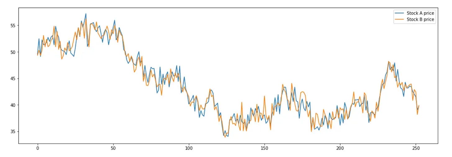
Before touching messy real-world markets, let’s build a small, clean sandbox. Suppose two stocks, A and B, are each driven by a shared latent factor F plus independent noise. If F follows a random walk and each stock is simply F + noise, then the stocks look like random walks on their own, but crucially, their difference behaves like noise around zero. That’s the essence of mean reversion in a spread.

In Python:

import numpy as np

np.random.seed(112)

# Shared factor: random walk
F = [50]
for i in range(252):
    F.append(F[i] + np.random.randn())
F = np.array(F)

# Prices as factor + idiosyncratic noise
P_a = F + np.random.randn(len(F))
P_b = F + np.random.randn(len(F))

Plot A and B on separate charts and both look like drunkards’ walks. Overlay them, however, and you’ll notice they tend to track each other closely. Now construct a market-neutral spread:

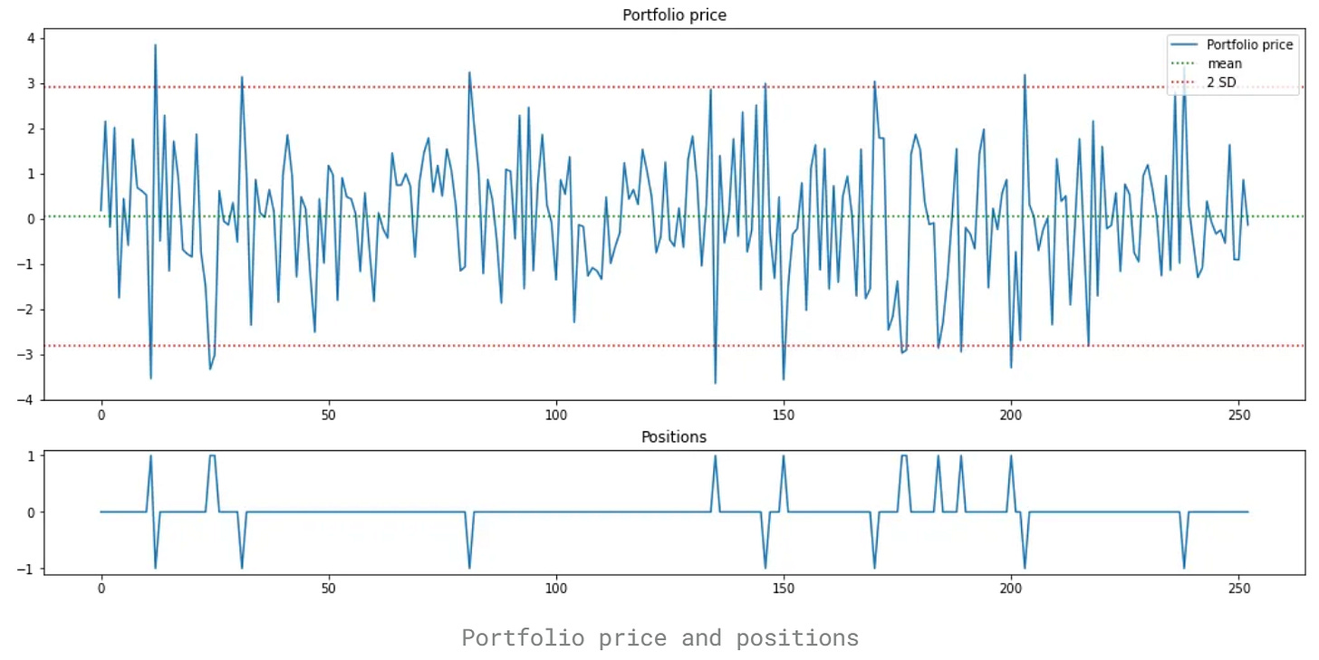
Spread_t = Price_A_t – Price_B_t

Because the common random-walk component cancels out, the spread jitters around zero, mean-reverting noise rather than a trending series.

From Intuition to Rules: A Simple Band Strategy

Once we have a spread with stationary behavior, turning it into a strategy is straightforward. Compute the spread’s rolling mean and standard deviation. Then:

1. Go long the spread (long A, short B) when the spread falls 2 standard deviations below its mean.

2. Close the long when the spread crosses back up through the mean.

3. Go short the spread (short A, long B) when the spread rises 2 standard deviations above its mean.

4. Close the short when the spread crosses down through the mean.

This is the Bollinger-band archetype for mean reversion. On our synthetic series, the rules generate a handful of sensible trades: the spread wanders, taps the bands, snaps back, and we monetize that snap.

Toy backtest takeaway. With a 1-share per leg position, our synthetic example produced ~15 trades and about $43 in total P&L (≈$2.87 per trade). Scale the position to 100 shares per leg and it’s about $4,300 exactly linear because we excluded costs, slippage, borrow fees, and execution constraints.

The point isn’t the dollar figure; it’s the logic chain:

common factor → stationary spread → band rules → monetizable reversion.

---